Sums and Limit Theorems of Random Variables

Many practical situations involve random variables defined as the sum or the average of other random variables. For example, estimating a population mean using a sample mean relies on the behavior of these sums and averages. Limit theorems provide the mathematical foundation that justifies such estimations.
Limit theorems describe how sums (or averages) of random variables behave as the number of terms increases. In this chapter, we focus on two key tools:

Concentration inequalities: they provide bounds on the probability that a random variable deviates significantly from its mean.
The Law of Large Numbers (LLN): it explains why averages stabilize: as an experiment is repeated many times, the average outcome approaches the theoretical expected value.

Modeling with Linear Combinations

In probability theory, we often analyze situations that arise from repeating the same experiment several times or from combining different random phenomena. To model them, we define new random variables as sums, averages, or more generally linear combinations of simpler random variables.
For instance, the total profit over a week is the sum of daily profits.

Definition Linear Combination of Random Variables

A linear combination of random variables $X_1, X_2, \ldots, X_n$ is a new random variable $Y$ defined by:$$ Y = a_1 X_1 + a_2 X_2 + \ldots + a_n X_n, $$where $a_1, a_2, \ldots, a_n$ are real constants.

Definition Sum and Mean of Random Variables

Given $n$ random variables $X_1, X_2, \dots, X_n$:

The sum is denoted $S_n = X_1 + X_2 + \ldots + X_n$.
The sample mean is denoted $\overline{X}_n = \dfrac{X_1 + X_2 + \ldots + X_n}{n}$.

Example

Suppose we roll two fair six-sided dice. Let $X_1$ be the result of the first die

and $X_2$ the result of the second die

The total score is $S_2 = X_1 + X_2$.
The average score is $\overline{X}_2 = \dfrac{X_1 + X_2}{2}$.

More generally, if we roll a die $n$ times and denote the outcomes by $X_1,\dots,X_n$, then $S_n$ models the cumulative score and $\overline{X}_n$ models the average score.

Expectation and Variance

When a random variable is defined as the sum or average of others, computing its full probability distribution can be very tedious (for example, finding the distribution of the sum of 100 dice).
Fortunately, thanks to the linearity of expectation and the additivity of variance (under independence), we can compute expectations and variances directly from the individual variables, without building the entire probability table of the result.

Proposition Properties of Expectation and Variance

For random variables $X, Y$ and real constants $a, b$:

Expectation is linear: for all $a,b\in\mathbb{R}$, $$ E(aX + bY) = aE(X) + bE(Y). $$
Variance adds for independent variables: if $X$ and $Y$ are independent, then $$ V(aX + bY) = a^2V(X) + b^2V(Y). $$

Example

Let $X_1$ and $X_2$ be the outcomes of rolling two fair six-sided dice. For one die, we know $E(X_1)=3.5$ and $V(X_1)=\dfrac{35}{12}\approx 2.92$.

The expected total score is $E(X_1+X_2)=E(X_1)+E(X_2)=3.5+3.5=7$.
Since the dice are independent, the variance of the total is $V(X_1+X_2)=V(X_1)+V(X_2)=\dfrac{70}{12}\approx 5.83$.

Proposition Expectation of Sums and Means

If $E(\overline{X}_i) = \mu$, for all $i$, then:$$ E(S_n) = n\mu \qquad\text{and}\qquad E(\overline{X}_n) = \mu. $$

Proof

By linearity of expectation:$$ \begin{aligned}E(S_n) &= E(X_1 + \cdots + X_n) = E(X_1) + \cdots + E(X_n) = n\mu,\\ E(\overline{X}_n) &= E\!\left(\frac{S_n}{n}\right) = \frac{1}{n}E(S_n) = \frac{n\mu}{n} = \mu.\end{aligned} $$

Example

If we roll $n=10$ dice, the expected average score per die remains $3.5$:$$ E(\overline{X}_{10}) = E(X_1) = 3.5. $$The expected total score is $E(S_{10}) = 10 \times 3.5 = 35$.

Proposition Variance of Sums and Means

If $X_1, X_2, \dots, X_n$ are independent and identically distributed with variance $\sigma^2$ (and standard deviation $\sigma$), then:

For the sum: $$ V(S_n) = n\sigma^2 \quad \text{and} \quad \sigma(S_n) = \sigma\sqrt{n}. $$
For the mean: $$ V(\overline{X}_n) = \frac{\sigma^2}{n} \quad \text{and} \quad \sigma(\overline{X}_n) = \frac{\sigma}{\sqrt{n}}. $$

Proof

By additivity of variance for independent variables and the property $V(aX)=a^2V(X)$:$$ \begin{aligned}V(S_n) &= V(X_1 + \cdots + X_n) = V(X_1) + \cdots + V(X_n) = n\sigma^2,\\ \sigma(S_n) &= \sqrt{V(S_n)} = \sqrt{n\sigma^2} = \sigma\sqrt{n},\\ V(\overline{X}_n) &= V\!\left(\frac{1}{n}S_n\right) = \frac{1}{n^2}V(S_n) = \frac{n\sigma^2}{n^2} = \frac{\sigma^2}{n},\\ \sigma(\overline{X}_n) &= \sqrt{V(\overline{X}_n)} = \sqrt{\frac{\sigma^2}{n}} = \frac{\sigma}{\sqrt{n}}.\end{aligned} $$

Example

Consider rolling $n=100$ dice. The variance of the average score $\overline{X}_{100}$ is:$$ V(\overline{X}_{100}) = \frac{V(X_1)}{100} = \frac{2.92}{100} = 0.0292. $$The standard deviation is $\sigma(\overline{X}_{100}) = \dfrac{\sigma(X_1)}{\sqrt{100}} = \dfrac{1.71}{10} = 0.171$.
Compared to a single die ($\sigma \approx 1.71$), the average of 100 dice is much less spread out and therefore much more stable (it concentrates around the expected value).

Concentration Laws

When we know the mean $\mu$ and the variance $V$ of a random variable, we often want to know how likely it is that the variable will take a value far away from its average.
Concentration inequalities provide a mathematical way to bound this probability. Unlike specific probability distributions, these inequalities work for any random variable, providing a "worst-case scenario" limit on the probability of a deviation. These inequalities are fundamental tools that we will use to rigorously prove the Law of Large Numbers.

Theorem Bienaymé-Tchebychev Inequality

Let $X$ be a random variable with mean $\mu$ and variance $V(X)$. For any real number $\delta>0$:$$ P\bigl(|X-\mu|\ge \delta\bigr)\le \frac{V(X)}{\delta^2}. $$This inequality provides an upper bound on the probability that $X$ deviates from its mean by at least $\delta$.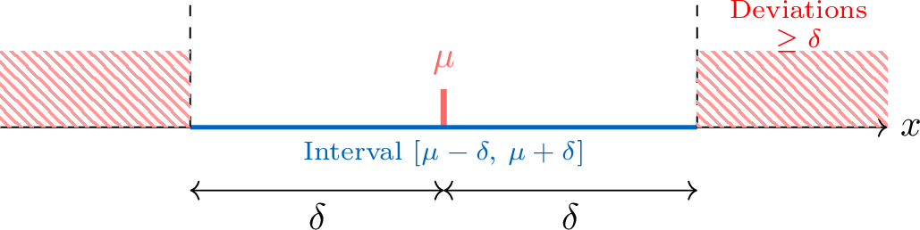

Example

A factory produces bags of sugar with mean weight $\mu=1000\,\text{g}$ and variance $V(X)=25$. We want to bound the probability that a bag differs from the mean by $10\,\text{g}$ or more.Here $\delta=10$. Applying the inequality:$$ P(|X-1000|\ge 10)\le \frac{25}{10^2}=\frac{25}{100}=0.25. $$There is at most a $25\,\pourcent$ chance that a bag lies outside the interval $[990,\,1010]$.

Proposition Concentration Inequality

Let $\overline{X}_n$ be the sample mean of $n$ independent and identically distributed variables, each with mean $\mu$ and variance $V$. For any $\delta>0$:$$ P\bigl(|\overline{X}_n-\mu|\ge \delta\bigr)\le \frac{V}{n\delta^2}. $$This shows that as $n$ increases, the probability that the average is far from $\mu$ tends to $0$.

Example

We toss a fair coin $n=1000$ times. Let $\overline{X}_n$ be the observed proportion of heads. Then $\mu=0.5$ and $V=0.25$. What is the probability that the proportion deviates from $0.5$ by more than $0.05$?Using the concentration inequality with $\delta=0.05$:$$ P(|\overline{X}_{1000}-0.5|\ge 0.05)\le \frac{0.25}{1000\times (0.05)^2}= \frac{0.25}{1000\times 0.0025}= \frac{0.25}{2.5}= 0.1. $$There is at most a $10\,\pourcent$ chance that the proportion lies outside $[0.45,\,0.55]$.

Law of Large Numbers

From an early age, we use experimental frequencies to estimate probabilities—for example, tossing a coin many times to test whether it is fair. The Law of Large Numbers provides a rigorous mathematical justification for this intuition: as the number of independent trials increases, the sample mean becomes a more and more reliable estimate of the theoretical expectation.

Theorem Law of Large Numbers

Let $X_1, X_2, \dots, X_n$ be independent and identically distributed random variables with mean $\mu$ and variance $V$. Let $\overline{X}_n$ be their sample mean. For any $\delta>0$:$$ \lim_{n\to\infty} P(|\overline{X}_n-\mu|\ge \delta)=0. $$In other words, for any fixed $\delta$, the probability that the sample mean deviates from $\mu$ by at least $\delta$ goes to $0$ as $n\to\infty$.

Proof

From the concentration inequality:$$ P(|\overline{X}_n-\mu|\ge \delta)\le \frac{V}{n\delta^2}. $$Since $V$ and $\delta$ are fixed, we have$$ \lim_{n\to\infty}\frac{V}{n\delta^2}=0. $$Because the probability is non-negative and bounded above by a sequence tending to $0$, the squeeze theorem gives$$ \lim_{n\to\infty} P(|\overline{X}_n-\mu|\ge \delta)=0. $$

Example

Consider tossing a fair coin ($p=0.5$). For $n=100$, the concentration inequality gives:$$ P(|\overline{X}_{100}-0.5|\ge 0.1)\le \frac{0.25}{100\times 0.1^2}=0.25. $$But for $n=1\,000\,000$:$$ P(|\overline{X}_{1\,000\,000}-0.5|\ge 0.1)\le \frac{0.25}{1\,000\,000\times 0.1^2}=0.000025. $$The average becomes extremely stable around the theoretical value as $n$ grows.