Discrete Random Variables
Random Variables
Definitions
Definition Random Variable
A random variable, denoted \(X\), is a function that assigns a numerical value to each outcome \(\omega\) in a random experiment. We write this value as \(X(\omega)\).
Example
Let \(X\) be the number of heads when tossing 2 fair coins:  (red coin) and
  (blue coin). Find \(X(\textcolor{colordef}{H},\textcolor{colorprop}{T})\).
The outcome \((\textcolor{colordef}{H},\textcolor{colorprop}{T})\) means the red coin shows heads (H) and the blue coin shows tails (T). Since \(X\) counts heads, there’s 1 head. Thus, \(X(\textcolor{colordef}{H},\textcolor{colorprop}{T}) = 1\).
Definition Discrete Random Variable
A random variable is discrete if its set of possible values is finite or countably infinite. This means we can list all possible values.
Definition Events Involving a Random Variable
For a random variable \(X\):
- \((X = x)\): The set of outcomes where \(X\) takes the value \(x\).
- \((X \leq x)\): The set of outcomes where \(X\) is less than or equal to \(x\).
- \((X \geq x)\): The set of outcomes where \(X\) is greater than or equal to \(x\).
Example
Let \(X\) be the number of heads when tossing 2 coins: and . List the outcomes for \((X = 0)\), \((X = 1)\), \((X = 2)\), \((X \leq 1)\), and \((X \geq 1)\).
- \((X = 0) = \{(\textcolor{colordef}{T},\textcolor{colorprop}{T})\}\) (no heads).
- \((X = 1) = \{(\textcolor{colordef}{T},\textcolor{colorprop}{H}), (\textcolor{colordef}{H},\textcolor{colorprop}{T})\}\) (one head).
- \((X = 2) = \{(\textcolor{colordef}{H},\textcolor{colorprop}{H})\}\) (two heads).
- \((X \leq 1) = (X = 0) \cup (X = 1) = \{(\textcolor{colordef}{T},\textcolor{colorprop}{T}), (\textcolor{colordef}{T},\textcolor{colorprop}{H}), (\textcolor{colordef}{H},\textcolor{colorprop}{T})\}\) (at most one head).
- \((X \geq 1) = (X = 1) \cup (X = 2) = \{(\textcolor{colordef}{T},\textcolor{colorprop}{H}), (\textcolor{colordef}{H},\textcolor{colorprop}{T}), (\textcolor{colordef}{H},\textcolor{colorprop}{H})\}\) (at least one head).
Probability Distribution
Definition Probability Distribution
The probability distribution of a random variable \(X\) lists the probability \(P(X = x_i)\) for each possible value \(x_1,x_2,\dots,x_n\). It can be shown as a table or formula.
Proposition Characteristic of a Probability Distribution
For a random variable \(X\) with possible values \(x_1,x_2,\dots,x_n\), we have
- \(0 \leq P(X=x_i) \leq 1\) for all \(i=1,\dots,n\),
- \(\displaystyle\sum_{i=1}^n P(X=x_i) =P(X=x_1)+P(X=x_2)+\dots+P(X=x_n)= 1 \).
Example
Let \(X\) be the number of heads when tossing 2 fair coins: and .
- List the possible values of \(X\).
- Find the probability distribution.
- Create the probability table.
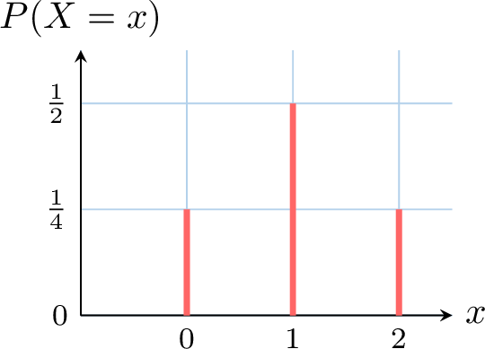
- Draw the probability distribution graph.
- Possible values: \(0\) (no heads), \(1\) (one head), \(2\) (two heads).
- Probability distribution:
- \(P(X = 0) = P(\{(\textcolor{colordef}{T},\textcolor{colorprop}{T})\}) = \frac{1}{4}\),
- \(P(X = 1) = P(\{(\textcolor{colordef}{T},\textcolor{colorprop}{H}), (\textcolor{colordef}{H},\textcolor{colorprop}{T})\}) = \frac{2}{4} = \frac{1}{2}\),
- \(P(X = 2) = P(\{(\textcolor{colordef}{H},\textcolor{colorprop}{H})\}) = \frac{1}{4}\).
- Probability table:
\(x\) 0 1 2 \(P(X = x)\) \(\frac{1}{4}\) \(\frac{1}{2}\) \(\frac{1}{4}\) - Graph:
Existence of a Random variable with a given Probability Distribution
Usually, defining a random variable begins by establishing:
- a sample space, that is, the set of all possible outcomes,
- a probability associated with this sample space,
- a function \(X\) that assigns a number to each outcome in the sample space.
| \(x\) | 0 | 1 | 2 | 3 |
| \(P(X = x)\) | \(\frac{10}{30}\) | \(\frac{12}{30}\) | \(\frac{5}{30}\) | \(\frac{3}{30}\) |
Theorem Existence of a Random Variable with a Given Probability Distribution
Suppose you have possible values \(x_1, x_2, \ldots, x_n\) and probabilities \(p_1, p_2, \ldots, p_n\).
If:
If:
- \(0 \leq p_i \leq 1\) for each \(i = 1, 2, \ldots, n\),
- \(\displaystyle\sum_{i=1}^n p_i = p_1 + p_2 + \cdots + p_n = 1\),
Method Defining a Random Variable \(X\) with a Valid Probability Distribution
In practice, we often define a random variable \(X\) directly by specifying its probability distribution. The key is to ensure that this distribution is valid, meaning it satisfies the conditions for a probability distribution: all probabilities must be non-negative and sum to 1.
Example
We survey a class of 30 students about their siblings and obtain these results: 10 students have 0 siblings, 12 have 1 sibling, 5 have 2 siblings, and 3 have 3 siblings. We define a random variable \(X\) as the number of siblings of a randomly chosen student, with this probability distribution:
| \(x\) | 0 | 1 | 2 | 3 |
| \(P(X = x)\) | \(\frac{10}{30}\) | \(\frac{12}{30}\) | \(\frac{5}{30}\) | \(\frac{3}{30}\) |
- \(P(X = x) \geq 0\) for all \(x = 0, 1, 2, 3\) (true: \(\frac{10}{30}\), \(\frac{12}{30}\), \(\frac{5}{30}\), and \(\frac{3}{30}\) are all non-negative),
- \(P(X = 0) + P(X = 1) + P(X = 2) + P(X = 3) = \frac{10}{30} + \frac{12}{30} + \frac{5}{30} + \frac{3}{30} = \frac{30}{30} = 1\) (true: the sum equals 1).
Measures of Center and Spread
Expectation
The expected value of a random variable \(X\) is the "average you’d expect if you repeated the experiment many times". It’s found by taking all possible values, multiplying each by its probability, and adding them up — essentially a weighted average where the probabilities act as the weights.
Definition Expected Value
For a random variable \(X\) with possible values \(x_1, x_2, \ldots, x_n\), the expected value, \(E(X)\), also called the mean, is:$$\begin{aligned}E(X) &= \sum_{i=1}^{n} x_i P(X = x_i)\\
&= x_1 P(X = x_1) + x_2 P(X = x_2) + \cdots + x_n P(X = x_n)\\
\end{aligned}$$
Example
You toss 2 fair coins, and \(X\) is the number of heads. The probability distribution is:
| \(x\) | 0 | 1 | 2 |
| \(P(X = x)\) | \(\frac{1}{4}\) | \(\frac{1}{2}\) | \(\frac{1}{4}\) |
Calculate \(E(X)\) using the formula:$$\begin{aligned}E(X) &= 0 \times \frac{1}{4} + 1 \times \frac{1}{2} + 2 \times \frac{1}{4} \\
&= \frac{1}{2} + \frac{2}{4} \\
&= 1\end{aligned}$$So, on average, you expect 1 head when tossing 2 coins.
Proposition Linearity of Expectation
For any random variable \(X\) and constants \(a\) and \(b\), the expected value of a linear transformation of \(X\) is:$$ E(aX + b) = aE(X) + b $$This property is derived from two simpler rules:
- \(E(aX) = aE(X)\) (The expectation of a scaled variable is the scaled expectation).
- \(E(X+b) = E(X) + b\) (The expectation of a shifted variable is the shifted expectation).
The following derivation relies on the formula for the expectation of a function of a discrete random variable, \(g(X)\), which is given by \(E(g(X)) = \sum g(x_i)P(X=x_i)\).
Let the function be \(g(X) = aX + b\).$$\begin{aligned}E(aX+b) &= \sum_{i} (ax_i + b) P(X=x_i) && \text{(by the formula for } E(g(X))\text{)} \\ &= \sum_{i} (ax_i P(X=x_i) + b P(X=x_i)) && \text{(distribute the probability)} \\ &= \sum_{i} ax_i P(X=x_i) + \sum_{i} b P(X=x_i) && \text{(split the summation)} \\ &= a \sum_{i} x_i P(X=x_i) + b \sum_{i} P(X=x_i) && \text{(factor out constants } a \text{ and } b\text{)} \\ &= a E(X) + b(1) && \text{(using } E(X) \text{ definition and } \sum P(X=x_i)=1\text{)} \\ &= aE(X) + b\end{aligned}$$
Let the function be \(g(X) = aX + b\).$$\begin{aligned}E(aX+b) &= \sum_{i} (ax_i + b) P(X=x_i) && \text{(by the formula for } E(g(X))\text{)} \\ &= \sum_{i} (ax_i P(X=x_i) + b P(X=x_i)) && \text{(distribute the probability)} \\ &= \sum_{i} ax_i P(X=x_i) + \sum_{i} b P(X=x_i) && \text{(split the summation)} \\ &= a \sum_{i} x_i P(X=x_i) + b \sum_{i} P(X=x_i) && \text{(factor out constants } a \text{ and } b\text{)} \\ &= a E(X) + b(1) && \text{(using } E(X) \text{ definition and } \sum P(X=x_i)=1\text{)} \\ &= aE(X) + b\end{aligned}$$
Variance and Standard Deviation
The variance measures how spread out the values of a random variable are from its expected value. The standard deviation is the square root of the variance, giving a sense of typical deviation in the same units as \(X\).
Definition Variance and Standard Deviation
The variance, denoted \(V(X)\), is:$$\begin{aligned}V(X) &= \sum_{i=1}^{n} (x_i - E(X))^2 P(X = x_i)\\
&= \left(x_1-E(X)\right)^2 P(X = x_1) + \left(x_2-E(X)\right)^2 P(X = x_2) + \cdots + \left(x_n-E(X)\right)^2 P(X = x_n)\\
\end{aligned}$$The standard deviation, denoted \(\sigma(X)\), is \(\sigma(X) = \sqrt{V(X)}\).
Example
You toss 2 fair coins, and \(X\) is the number of heads. The probability table is:
| \(x\) | 0 | 1 | 2 |
| \(P(X = x)\) | \(\frac{1}{4}\) | \(\frac{1}{2}\) | \(\frac{1}{4}\) |
Calculate \(V(X)\):$$\begin{aligned}V(X) &= (0 - 1)^2 \times \frac{1}{4} + (1 - 1)^2 \times \frac{1}{2} + (2 - 1)^2 \times \frac{1}{4} \\
&= 1 \times \frac{1}{4} + 0 \times \frac{1}{2} + 1 \times \frac{1}{4} \\
&= \frac{1}{4} + 0 + \frac{1}{4} \\
&= \frac{1}{2} \\
\end{aligned}$$The variance is \(\frac{1}{2}\).
Proposition Computational Formula for Variance
A more convenient formula for computation is:$$V(X) = E(X^2) - [E(X)]^2$$
Let \(\mu = E(X)\).$$\begin{aligned}V(X) &= E[(X - \mu)^2] \\
&= E[X^2 - 2\mu X + \mu^2] \\
&= E(X^2) - E(2\mu X) + E(\mu^2) && \text{(by linearity of expectation)} \\
&= E(X^2) - 2\mu E(X) + \mu^2 && \text{(since } \mu \text{ and } \mu^2 \text{ are constants)} \\
&= E(X^2) - 2\mu(\mu) + \mu^2 \\
&= E(X^2) - 2\mu^2 + \mu^2 \\
&= E(X^2) - \mu^2 \\
&= E(X^2) - [E(X)]^2\end{aligned}$$
Classical Distributions
Uniform Distribution
Definition Uniform Distribution
A random variable \(X\) follows a uniform distribution if each possible value has the same probability:$$P(X = x) = \frac{1}{\text{Number of possible values}}, \quad \text{for any possible value }x$$
Example
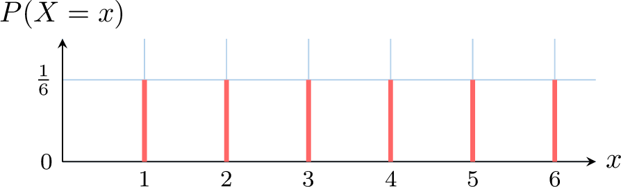
Let \(X\) be the result of rolling a fair die:  .
.
- List the possible values of \(X\).
- Create the probability table.
- Draw the probability distribution graph.
- Possible values: \(1, 2, 3, 4, 5, 6\).
- Probability table:
\(x\) 1 2 3 4 5 6 \(P(X = x)\) \(\frac{1}{6}\) \(\frac{1}{6}\) \(\frac{1}{6}\) \(\frac{1}{6}\) \(\frac{1}{6}\) \(\frac{1}{6}\) - Graph:
Proposition Expectation and Variance of a Uniform Distribution
For a random variable \(X\) that follows a uniform distribution on the set of integers \(\{1, 2, \ldots, n\}\):
- The expected value is \(E(X) = \frac{n+1}{2}\).
- The variance is \(V(X) = \frac{n^2-1}{12}\).
Proof of the Expected Value \(E(X)\):For a uniform distribution on \(\{1, 2, \dots, n\}\), the probability of any outcome is \(P(X=i) = \frac{1}{n}\). $$ \begin{aligned} E(X) &= \sum_{i=1}^n i \cdot P(X=i) \\
&= \sum_{i=1}^n i \cdot \frac{1}{n} \\
&= \frac{1}{n} \sum_{i=1}^n i \quad \text{(factoring out the constant } 1/n\text{)} \\
&= \frac{1}{n} \left( \frac{n(n+1)}{2} \right) \quad \text{(using the formula for the sum of integers)} \\
&= \frac{n+1}{2} \end{aligned} $$
Example
Let \(X\) be the random variable for the score on a roll of a fair six-sided die. Find the mean and variance of \(X\).
The random variable \(X\) follows an uniform distribution on \(\{1, 2, 3, 4, 5, 6\}\).
- \( E(X) = \frac{6+1}{2} = 3.5 \)
- \( V(X) = \frac{6^2-1}{12} = \frac{35}{12} \approx 2.92 \)
Bernoulli Distribution
A Bernoulli distribution models an experiment with two outcomes: success (1) or failure (0), like flipping a coin where heads is 1 and tails is 0. The probability of success is \(p\).
Definition Bernoulli Distribution
A random variable \(X\) follows a Bernoulli distribution if:
- Possible values are 0 and 1.
- \(P(X = 1) = p\) and \(P(X = 0) = 1 - p\).
Example
A basketball player has an 80\(\pourcent\) chance of making a free throw. Let \(X = 1\) if the shot is made, and \(X = 0\) if it’s missed.
- Is \(X\) a Bernoulli random variable?
- Find the probability of success.
- Yes, \(X\) has values 0 or 1, so it follows a Bernoulli distribution.
- Probability of success: \(P(X = 1) = 80\pourcent = 0.8\).
Proposition Expectation and Variance of a Bernoulli Distribution
For a Bernoulli random variable \(X\) with a probability of success \(p\), the following hold:
- The expected value is \(E(X) = p\),
- The variance is \(V(X) = p(1 - p)\),
- The standard deviation is \(\sigma(X) = \sqrt{p(1 - p)}\).
- \(\begin{aligned}[t]E(X)&=0\times P(X=0)+1\times P(X=1)\\&=0\times(1-p)+1\times p\\&=p\end{aligned}\)
- \(\begin{aligned}[t] V(X) &= (0-p)^2(1-p) + (1-p)^2 p \\ &= p^2(1-p) + p(1-p)^2 \\ &= p(1-p) [p + (1-p)] \\ &= p(1-p) \\ \end{aligned} \)
Binomial Distribution
Suppose a basketball player takes \(n\) free throws, and we count the number of shots made. The probability of making a free throw is the same for each attempt, and each shot is independent of every other shot. This is an example of a binomial experiment.
Definition Binomial Experiment
A binomial experiment is a statistical experiment that consists of a sequence of repeated Bernoulli trials. It must satisfy the following four conditions:
- Fixed Number of Trials: The experiment consists of a fixed number of trials, denoted by \(n\).
- Independent Trials: The outcome of each trial is independent of the outcomes of all other trials.
- Two Outcomes: Each trial has only two possible outcomes, typically labeled "success" and "failure".
- Constant Probability: The probability of success, denoted by \(p\), is the same for each trial. The probability of failure is \(1-p\).
Proposition Distribution of a Binomial Random Variable
Let \(X\) be a binomial random variable with \(n\) independent trials and a probability of success \(p\). The probability distribution of \(X\) is: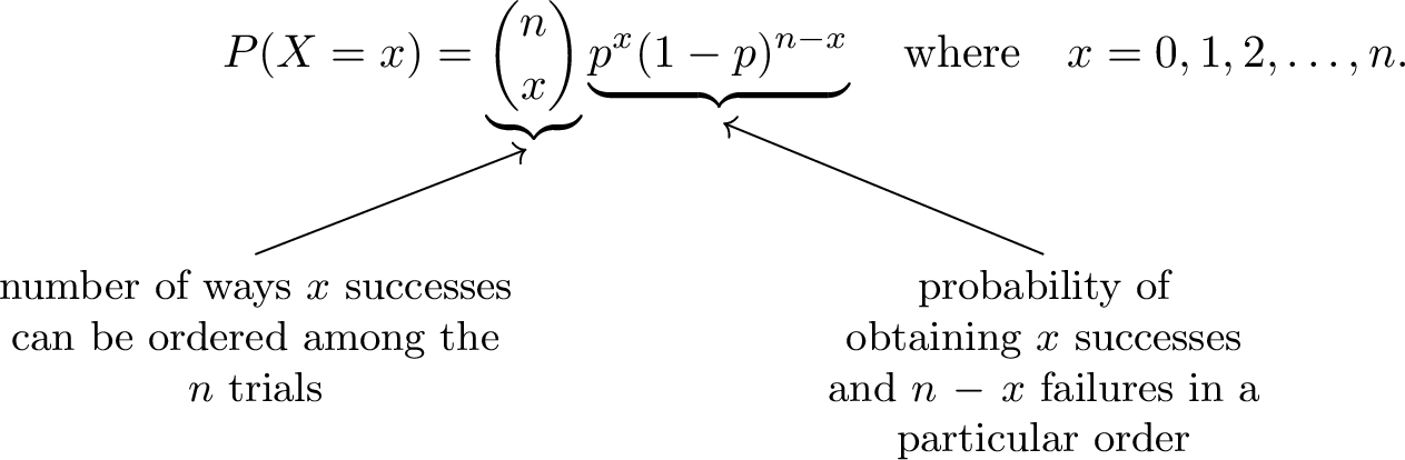
Consider the case where \(n = 3\). Let \(X_1\), \(X_2\), and \(X_3\) be three independent Bernoulli random variables, each with a probability of success \(p\). Define \(X = X_1 + X_2 + X_3\), which represents a binomial random variable.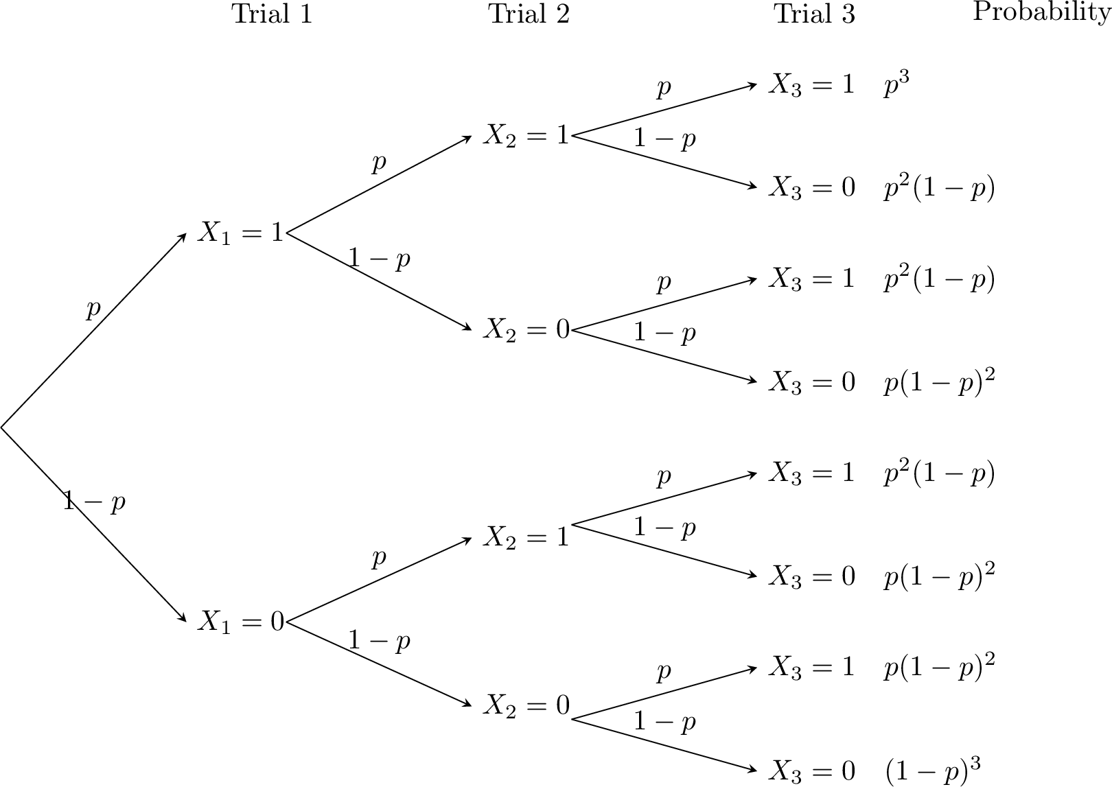
The logic generalizes for any \(n\). To obtain exactly \(x\) successes, we must choose \(x\) of the \(n\) trials to be successes, which can be done in \(\binom{n}{x}\) ways. Each specific arrangement of \(x\) successes and \(n-x\) failures has a probability of \(p^x (1-p)^{n-x}\). By the addition rule, the total probability is the sum over all these arrangements, resulting in \(P(X=x) = \binom{n}{x}p^x (1-p)^{n-x}\).
- The possible values of \(X\) are \(0, 1, 2, 3\).
- Probability calculations:
- \(\begin{aligned}[t] P(X = 0) &= P(X_1 = 0 \text{ and } X_2 = 0 \text{ and } X_3 = 0) \\ &= P(X_1 = 0) P(X_2 = 0) P(X_3 = 0) \quad \text{(since \)X_1, X_2, X_3\( are independent)} \\ &= (1-p)^3 \\ &= \binom{3}{0} p^0 (1-p)^3 \end{aligned}\)
- \(\begin{aligned}[t] P(X = 1) &= P(X_1 = 1 \text{ and } X_2 = 0 \text{ and } X_3 = 0) + P(X_1 = 0 \text{ and } X_2 = 1 \text{ and } X_3 = 0) \\ &\quad + P(X_1 = 0 \text{ and } X_2 = 0 \text{ and } X_3 = 1) \\ &= p (1-p)^2 + p (1-p)^2 + p (1-p)^2 \\ &= 3 p (1-p)^2 \\ &= \binom{3}{1} p^1 (1-p)^2 \end{aligned}\)
- \(\begin{aligned}[t] P(X = 2) &= P(X_1 = 1 \text{ and } X_2 = 1 \text{ and } X_3 = 0) + P(X_1 = 1 \text{ and } X_2 = 0 \text{ and } X_3 = 1) \\ &\quad + P(X_1 = 0 \text{ and } X_2 = 1 \text{ and } X_3 = 1) \\ &= p^2 (1-p) + p^2 (1-p) + p^2 (1-p) \\ &= 3 p^2 (1-p) \\ &= \binom{3}{2} p^2 (1-p)^1 \end{aligned}\)
- \(\begin{aligned}[t] P(X = 3) &= P(X_1 = 1 \text{ and } X_2 = 1 \text{ and } X_3 = 1) \\ &= p^3 \\ &= \binom{3}{3} p^3 (1-p)^0 \end{aligned}\)
The logic generalizes for any \(n\). To obtain exactly \(x\) successes, we must choose \(x\) of the \(n\) trials to be successes, which can be done in \(\binom{n}{x}\) ways. Each specific arrangement of \(x\) successes and \(n-x\) failures has a probability of \(p^x (1-p)^{n-x}\). By the addition rule, the total probability is the sum over all these arrangements, resulting in \(P(X=x) = \binom{n}{x}p^x (1-p)^{n-x}\).
Example
A basketball player has an 80\(\pourcent\) chance of making a free throw and takes 5 shots. Let \(X\) be the number of shots made.
- Is \(X\) a binomial random variable?
- Find the probability of making 4 shots.
- Yes, \(X\) is a binomial random variable because it counts the number of successes (shots made) in 5 independent trials (free throws), each with a constant success probability of 0.8.
- As \(X \sim B(5, 0.8)\), $$ \begin{aligned} P(X = 4) &= \binom{5}{4} (0.8)^4 (1-0.8)^1 \\ &= 5 \times 0.4096 \times 0.2 \\ &= 0.4096 \end{aligned} $$ The probability of making 4 shots is 0.4096.
Proposition Expectation and Variance of a Binomial Random Variable
For \(X \sim B(n, p)\):
- \(E(X) = n p\) (expected value),
- \(V(X) = n p (1 - p)\) (variance),
- \(\sigma(X) = \sqrt{n p (1 - p)}\) (standard deviation).
Example
A basketball player has an 80\(\pourcent\) chance of making a free throw and takes 5 shots. Find the mean and standard deviation of the number of successful shots.
Let \(X\) be the number of successful shots. Since each shot is independent and has a success probability of 0.8, we have \(X \sim B(5, 0.8)\).$$\begin{aligned}E(X) &= 5 \times 0.8 = 4, \\
V(X) &= 5 \times 0.8 \times (1 - 0.8) = 5 \times 0.8 \times 0.2 = 0.8, \\
\sigma(X) &= \sqrt{0.8} \approx 0.89.\end{aligned}$$Mean is 4 successful shots, standard deviation is about 0.89.