Statistics
Statistical Investigation
A step-by-step guide
Turn on the TV or flip through a newspaper, and you’ll often spot statistics in action. For example:
- Su averages 14.6 points per basketball game.
- Last year was the hottest on record since 1897.
- Scientific Research: Testing if a new medicine works by studying trial results.
- Industrial Production: Improving products by tracking defects and fixing processes.
- Social Issues: Figuring out what people think about new laws through surveys.
- Step 1: State the Problem: Decide what you want to learn.
Example: How has the average temperature changed over the last 100 years? - Step 2: Collect Data: Gather the info you need.
Example: Get temperature records from weather stations. - Step 3: Calculate Descriptive Statistics: Summarize the data with tools like mean, median, or mode.
Example: Find the average temperature for each decade. - Step 4: Organize and Display Data: Put the data in order and show it with charts or graphs.
Example: Make a graph of temperature changes over time. - Step 5: Interpret the Statistics: Figure out what the data tells you.
Example: Does the data show temperatures are rising significantly?
Definition Statistics
Statistics is all about collecting information, sorting it out, summarizing it, and figuring out what it means.
Stating the Problem
Population
When you start a statistical investigation, the first step is to ask a clear question. This keeps you focused on what you’re trying to find out and who or what you’re studying.
We call the group we’re studying the population. It could be all the people in a country, every student in a school, all the animals of a species, or even every item made by a machine. The information we collect from this group is called data, and it can come in many forms—like numbers, words, or measurements.
We call the group we’re studying the population. It could be all the people in a country, every student in a school, all the animals of a species, or even every item made by a machine. The information we collect from this group is called data, and it can come in many forms—like numbers, words, or measurements.
Definition Problem
A problem in statistics is a question that guides us to the information we need to find.
Example
Do girls like math more than boys?
Definition Population
A population is the whole group of people or things with something in common that we want to study.
Example
The population is all the students in a college.
Data
Definition Data
Data is the information we collect, like numbers, words, measurements, or observations.
Example
For our math study, we collect:
- Gender: Is the student a boy or a girl?
- Favorite Subject: What subject do they like best (e.g., Math, Science, English)?
- Math test score: What was their grade on the last assessment??
Definition Types of Variables
- Qualitative Variable (Categorical): Describes categories or groups that cannot be measured numerically.
- Quantitative Variable (Numerical): Represents measurable quantities with numerical values.
Example
For our math study:
- Qualitative Variables: Gender and favorite subject.
- Quantitative Variable: Math test score.
Collecting Data
Sampling
To collect data, we first decide who or what we’re asking. We can either:
- Do a census: Ask every single member of the population.
- Do a survey: Ask just a part of the population (a sample).
Definition Census
A census means collecting data from everyone in the population.
Definition Survey
A survey means collecting data from a smaller group (sample) of the population.
Example
If you ask every student in the collège about their favorite subject, is it a census or a survey?
It’s a census.
Example
If you only ask the students who are in class math today, is it a census or a survey?
It’s a survey.
Statistical Error in Sampling
One of the most common ways to collect information about a large group is to use a sample.For a sample to be meaningful, it must fairly represent the entire population.Two key challenges in sampling are: avoiding bias and ensuring the sample is large enough to capture the population’s diversity.
- Selection bias: A famous example of biased sampling is the Literary Digest poll before the 1936 U.S. presidential election.The magazine sent millions of surveys using telephone books and car registration lists. But during the Great Depression, many people couldn’t afford phones or cars.This led to a sample biased toward wealthier citizens, who were more likely to vote Republican.As a result, the poll incorrectly predicted a landslide win for Alfred Landon, while Franklin D. Roosevelt won by a wide margin.
- Sample size: During the Cuban Missile Crisis of 1962, U.S. intelligence underestimated the number and types of Soviet missiles in Cuba due to limited reconnaissance data.The small “sample” of photos led analysts to miss several launch sites, including those with longer-range missiles.This example shows how insufficient data can lead to serious misjudgments, especially when the stakes are high.
Definition Statistical Error
A statistical error is the difference between the observed result (from the sample) and the actual value (in the population).
Definition Selection Bias
Selection bias occurs when the sampling method makes some individuals in the population less likely to be included than others.
Proposition Random Sampling
If each member of the population is selected randomly, selection bias is avoided.
Proposition Sample Size
As the sample size increases, the statistical error generally decreases—our results become more accurate.
Descriptive Statistics
A Statistic
Descriptive statistics are numbers that help us summarize and understand data—like finding the average or the most common answer.
Definition A statistics
A statistics is a single value that sums up or describes a set of data.
Example
The average score in a class is 85\(\pourcent\) is a statistics number because it tells us something about the whole group in one simple figure.
Relative Frequency
In statistics, it’s important to understand the frequency of a category. This concept helps us analyze patterns and make predictions. It applies to everyday scenarios, such as gauging the popularity of a favorite food among friends or calculating how often a basketball player scores a shot. By studying relative frequencies, we gain valuable insights into data trends.
Definition Frequency and Relative Frequency
Frequency is how many times each value or category appears.
Relative Frequency is the frequency divided by the total, often shown as a percentage.
Relative Frequency is the frequency divided by the total, often shown as a percentage.
Example
The data for favorite subject is: Maths: 15 students, Sciences: 12 students, English: 3 students.
Fill in the table:
Fill in the table:
| Subject | Frequency | Relative frequency (\(\pourcent)\) |
| Maths | ||
| Sciences | ||
| English | ||
| Total | \(100 \pourcent\) |
| Subject | Frequency | Relative frequency (\(\pourcent)\) |
| Maths | 15 | \(\frac{15}{30}\times 100\pourcent = 50\pourcent\) |
| Sciences | 12 | \(\frac{12}{30}\times 100\pourcent = 40\pourcent\) |
| English | 3 | \(\frac{3}{30}\times 100\pourcent = 10\pourcent\) |
| Total | 30 | \(100 \pourcent\) |
Central Tendency
In statistics, central tendency refers to a measure that identifies a single value as representative of the center or typical point of a dataset. Three key measures are commonly used to assess central tendency: the mode, the mean, and the median.
Definition Mode
The mode is the value that shows up most often in your data.
Example
A group of students reported their last mark (out of 5) on a math exam as follows:$$ 1, 4, 2, 3, 5, 4, 5, 4, 3 $$What is the mode of this dataset?
From the frequency table:
| Mark | Frequency |
| 1 | 1 |
| 2 | 1 |
| 3 | 2 |
| 4 | 4 |
| 5 | 2 |
Definition Mean
The mean is the average. Add up all the values and divide by how many there are:$$\begin{aligned}\bar{x} &= \frac{\text{sum of all values}}{\text{number of values}} \\&= \frac{x_1 + x_2 + x_3 + \dots + x_n}{n}\end{aligned}$$
Example
Ratings: 1, 4, 2, 3, 5, 4, 5, 4, 4. What’s the mean?
$$\begin{aligned}\text{Mean} &= \frac{1 + 4 + 2 + 3 + 5 + 4 + 5 + 4 + 4}{9} \\&= \frac{32}{9}\\& \approx 3.56\end{aligned}$$
Definition Median
The median is the middle value when you line up the data from smallest to largest:
- If there’s an odd number of values, it’s the one in the middle.
- If there’s an even number, average the two middle values.
Example
Ratings: 1, 4, 2, 3, 5, 4, 5, 4, 4. What’s the median?
The ordered set is:$$1,2,3,4,\textcolor{colorprop}{4},4,4,5,5$$The middle value is \(\textcolor{colorprop}{4}\), so the median is \(\textcolor{colorprop}{4}\).
Dispersion
When analyzing data, it's not only important to understand the central tendency—which refers to the typical value of a dataset (such as the mean, median, or mode)—but also to examine how much the data varies. This variation is called dispersion.
While measures of central tendency summarize the center of the data, measures of dispersion tell us how spread out the values are.To illustrate this, let’s look at the test scores of two students:
While measures of central tendency summarize the center of the data, measures of dispersion tell us how spread out the values are.To illustrate this, let’s look at the test scores of two students:
- Student A's scores: 10, 50, 90
- Student B's scores: 45, 50, 55
- Student A’s scores: show a wide variation, ranging from 10 to 90.
- Student B’s scores: are much more concentrated, between 45 and 55.
Definition Range
The range is the difference between the maximum and minimum values in a dataset.$$\text{range} = \text{maximum} - \text{minimum}$$
Example
Find the range for the following data: \(1,19,10,2,18,10,5,15,10\).
The minimum value is 1 and the maximum is 19.
So, the range is \(19 - 1 = 18\).
So, the range is \(19 - 1 = 18\).
Definition Quartile
Quartiles are values that divide an ordered dataset into four equal parts.
The median splits the data into two halves. The quartiles divide these halves again, giving us four equal parts.
Definition Interquartile Range
The interquartile range (IQR) is the difference between the upper quartile (Q3) and the lower quartile (Q1).$$\text{interquartile range} = \text{Q3} - \text{Q1}$$
Example
Find the quartiles and the interquartile range for the following data:$$1,19,10,2,18,10,5,15,10$$
- Order the data: $$1, 2, 5, 10, \textcolor{colorprop}{10}, 10, 15, 18, 19$$
- The median (Q2) is 10.
- The lower half (before the median): \(1,\textcolor{colorprop}{2,5},10\) → \(Q_1 = \frac{2+5}{2} = 3.5\)
- The upper half (after the median): \(10,\textcolor{colorprop}{15,18},19\) → \(Q_3 = \frac{15+18}{2} = 16.5\)
- So, the interquartile range is \(16.5 - 3.5 = 13\)
Organizing and Displaying Data
Visualizing frequencies
In statistics, graphs help us quickly understand how categories compare. Two common tools are:
- Bar charts use rectangular bars. Their length shows the frequency of each category. They are ideal for comparing categories side by side.
- Pie charts divide a circle into slices. Each slice represents a proportion of the total. They are useful for showing how parts make up a whole.
Definition Bar Chart/Histogram
A bar chart/histogram shows data with bars:
- Categories or values go on \(x\)-axis.
- Frequencies go on \(y\)-axis.
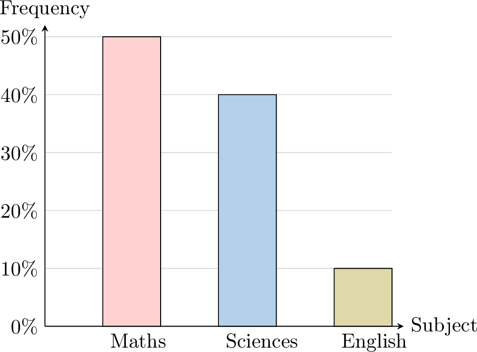
Example
Draw a bar chart for:
| Subject | Relative frequency (\(\pourcent)\) |
| Maths | \(50\pourcent\) |
| Sciences | \( 40\pourcent\) |
| English | \( 10\pourcent\) |
Definition Pie Chart
A pie chart is a circle split into slices to show how data compares.
Example
Draw the pie chart of the following data:
| Subject | Frequency |
| Maths | 15 |
| Sciences | 12 |
| English | 3 |
| Total | 30 |
Angles are :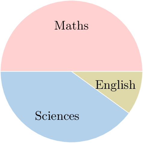
- Maths : \(\frac{15}{30} \times 360^\circ = 180^\circ\)
- Sciences : \(\frac{12}{30} \times 360^\circ = 144^\circ\)
- English : \(\frac{3}{30} \times 360^\circ = 36^\circ\)
Visualizing Central Tendency and Dispersion
In statistics, it's important to understand where the data is centered and how spread out it is. To show both aspects clearly, we use visual tools.
- Central tendency refers to the middle of the data, often represented by the mean, median, or mode.
- Dispersion shows how much the data varies, using measures like range or interquartile range.
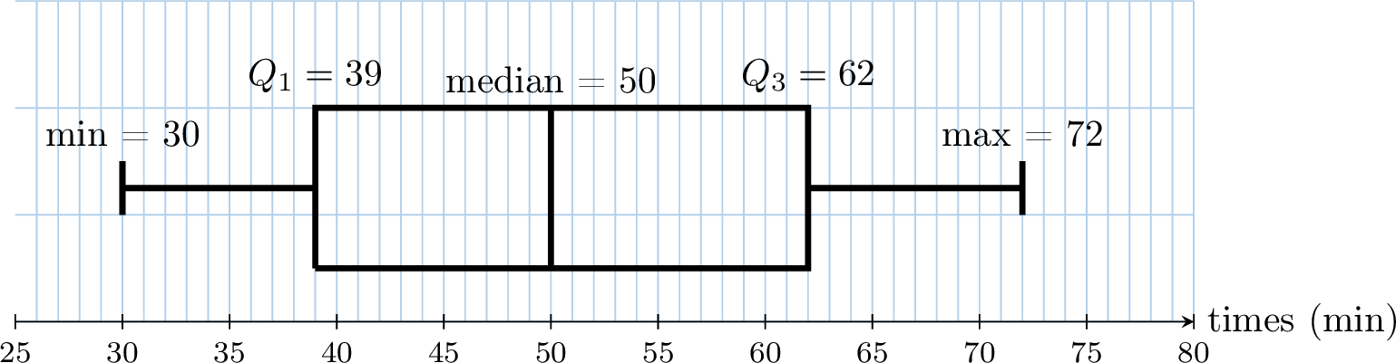
Definition Box plot (whisker plot)
A whisker plot, also called a box plot, displays the five-number summary of a set of data. The five-number summary is the minimum, first quartile, median, third quartile, and maximum.
In a box plot, we draw a box from the first quartile to the third quartile. A vertical line goes through the box at the median. The whiskers go from each quartile to the minimum or maximum.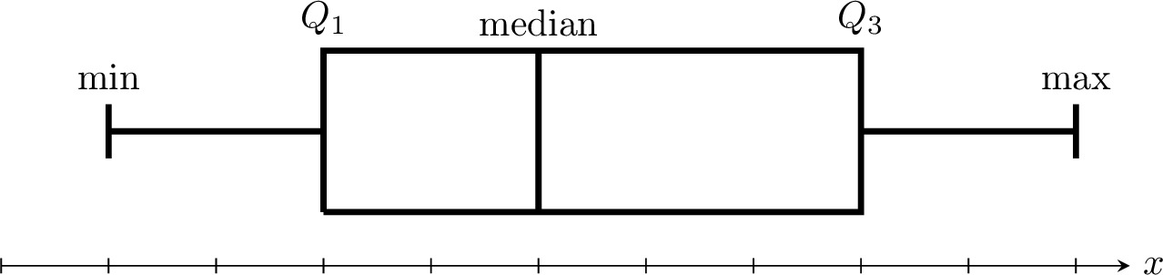
In a box plot, we draw a box from the first quartile to the third quartile. A vertical line goes through the box at the median. The whiskers go from each quartile to the minimum or maximum.
Example
This box plot shows the number of minutes passengers spent in an airport departure lounge. What is the minimum number of minutes spent waiting in the lounge?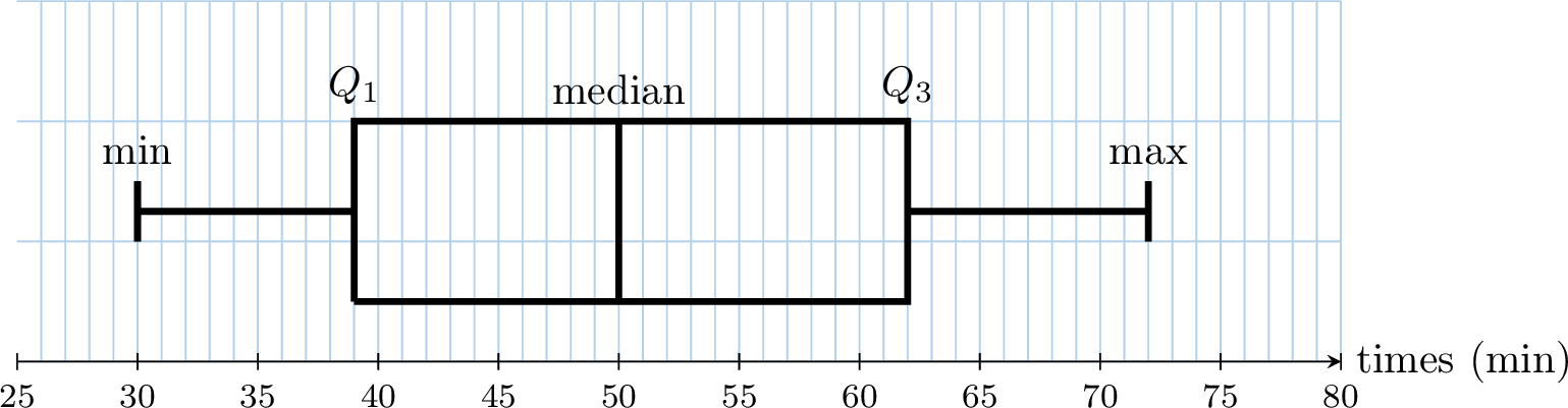
Interpreting the Statistics
Reading and Comparing Data
Interpreting statistics means turning raw data into meaningful insights that help us understand the world and make informed decisions. This involves reading tables, analyzing graphs, and comparing values such as averages, frequencies, and measures of spread.
Visual tools like pie charts or bar graphs make patterns easier to spot, while comparisons (using mean, median, or interquartile range) help highlight differences between groups.
Visual tools like pie charts or bar graphs make patterns easier to spot, while comparisons (using mean, median, or interquartile range) help highlight differences between groups.
Example
This pie chart shows the favorite subjects of students:
The largest section corresponds to Maths, so it is the most popular subject.
Example
The girls' average score in math is 87 (B+), while the boys' average is 75 (C). Are girls better at math?
Yes, since 87 > 75, on average, girls perform better than boys in math.