Exponential Functions
In previous chapters, we explored how to evaluate expressions of the form \(a^n\) where \(n\) is an integer or rational number. This chapter extends that understanding to the exponential function \(f(x) = a^x\), where \(x\) can be any real number. We will examine its graphical representation, properties, and applications in modeling real-world phenomena such as population growth and compound interest.
Exponential Function
Definition Exponential Function
The exponential function has the form \(f(x)=a^x\) where \(a>0, a \neq 1\).
Example
For the graph of the exponential function \(f(x)=2^x\),
- Complete the table of values
\(x\) \(-3\) \(-2\) \(-1\) 0 1 2 3 \(f(x)\) - Sketch the graph.
-
\(x\) \(-3\) \(-2\) \(-1\) 0 1 2 3 \(f(x)\) \(\frac{1}{8}\) \(\frac{1}{4}\) \(\frac{1}{2}\) 1 2 4 8 -
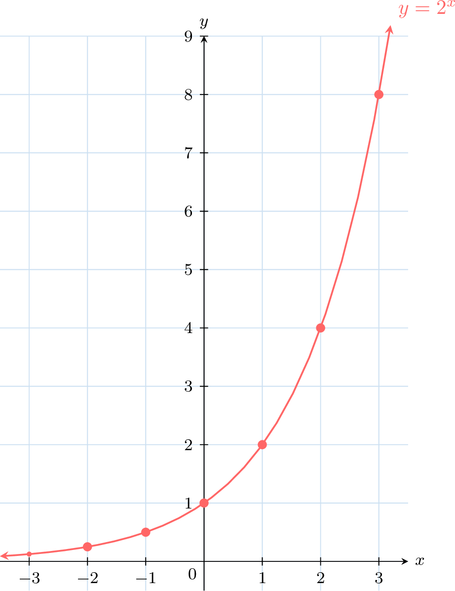
All exponential graphs are similar in shape and have a horizontal asymptote.
Proposition Exponential Function Shape
For the shape of the exponential function \(x\mapsto a^{x}\):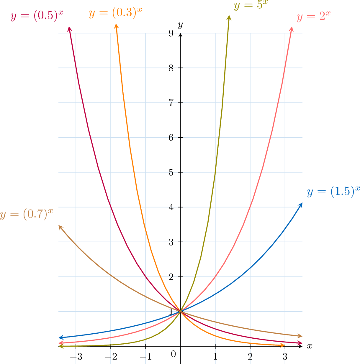
- \(a\) controls how steeply the graph increases or decreases
- \(a>1\) the function is increasing.
- \(0 \lt a\lt 1\) the function is decreasing.
Exponential vs. Linear Relationships
Proposition Exponential vs. linear relationships
If the difference between \(x\)-values is constant, then
- in a linear relationship, the difference between \(y\)-values is constant.
- in an exponential relationship, the ratio between \(y\)-values is constant.
- Let \(y=a x +b\) a linear relationship.
Let \(k\) the constant difference between \(x_2\) and \(x_1\). So \( x_2 -x_1=k\).
Let \(y_1 = a x_1 +b\) and \(y_2 = a x_2 +b\).
The difference between between \(y_2\) and \(y_1\) is:$$\begin{aligned}[t]y_2-y_1&= (a x_2 +b)-(a x_1 +b)\\ &=a(x_2-x_1)\\ &=ak\\ \end{aligned}$$So the difference of between \(y\)-values is constant. - Let \(y=c a^{x}\) an exponential relationship.
Let \(k\) the constant difference between \(x_2\) and \(x_1\). So \( x_2 -x_1=k\).
Let \(y_1 = c a^{x_1}\) and \(y_2 = c a^{x_2}\).
The ratio between \(y_2\) and \(y_1\) is:$$\begin{aligned}[t]\frac{y_2}{y_1}&= \frac{c a^{x_2}}{c a^{x_1}}\\ &=a^{x_2-x_1}\\ &=a^k\\ \end{aligned}$$So the ratio between \(y\)-values is constant.
Example
Consider the relationship represented by this table:
| \(x\) | 0 | 1 | 2 | 3 |
| \(y\) | 0 | 20 | 40 | 60 |
For each increase of \(1\) in \(x\), the value of \(y\) increases by \(20\).$$\begin{aligned}x: &\ 0 & \textcolor{colordef}{\xrightarrow{\;+1\;}} & 1 & \textcolor{colordef}{\xrightarrow{\;+1\;}} & 2 & \textcolor{colordef}{\xrightarrow{\;+1\;}} & 3\\
y: &\ 0 & \textcolor{colorprop}{\xrightarrow{\;+20\;}} & 20 & \textcolor{colorprop}{\xrightarrow{\;+20\;}} & 40 & \textcolor{colorprop}{\xrightarrow{\;+20\;}} & 60\\
\end{aligned}$$So, this relationship is linear (\(y=20x\)).
Example
Consider the relationship represented by this table:
| \(x\) | 0 | 1 | 2 | 3 |
| \(y\) | 2 | 4 | 8 | 16 |
For each increase of \(1\) in \(x\), the value of \(y\) is multiplied by \(2\).$$\begin{aligned}x: &\ 0\ & \textcolor{colordef}{\xrightarrow{\;+1\;}} &\ 1\ & \textcolor{colordef}{\xrightarrow{\;+1\;}} &\ 2\ & \textcolor{colordef}{\xrightarrow{\;+1\;}} &\ 3 \\
y: &\ 2\ & \textcolor{colorprop}{\xrightarrow{\;\times 2\;}} &\ 4\ & \textcolor{colorprop}{\xrightarrow{\;\times 2\;}} &\ 8\ & \textcolor{colorprop}{\xrightarrow{\;\times 2\;}} &\ 16 \\
\end{aligned}$$So, this relationship is exponential (\(y = 2 \times 2^x\)).
Exponential Models
Exponential functions model a relationship in which a constant change in the independent variable gives the same proportional change in the dependent variable. This occurs widely in the natural and social sciences, as in a self-reproducing population, a fund accruing compound interest, or a growing body of manufacturing expertise. Thus, the exponential function also appears in a variety of contexts within physics, computer science, chemistry, engineering, mathematical biology, and economics.
For example, if a population of bacteria doubles every second, we would have 1, then 2, then 4, then 8, 16, 32, 64, 128, 256, etc! With this, we can observe the manner of exponential growth in bacteria. So the population after \(n\) seconds is \(P(n)=2^n\).
We expect that the population will actually grow in a smooth curve rather than in discrete jumps. So the population after \(t\) seconds is \(P(t)=2^t\).
Definition Base Model for Exponential Growth and Decay
A continuous exponential growth and decay has the form \(f(t)=k a^t\).
A discrete exponential growth and decay has the form \(u_n=k a^n\).
A discrete exponential growth and decay has the form \(u_n=k a^n\).
Example
The population of foxes, \(P\), in a specified area, \(t\) years after observation began, is modeled by the equation: \(P(t)=300(1.25)^t\).
- How many foxes are there initially?
- How many foxes are there after 5 years?
- The initial time is \(t=0\). So, the number of foxes is:$$\begin{aligned}P(0) &=300(1.25)^0 \\ &=300 \times 1 \\ &=300 \text { foxes }\end{aligned}$$
- Substitute \(t=5\) into the equation and round the final answer to the nearest fox, we find$$\begin{aligned}P(5) &=300(1.25)^5 \\ & =300 \times \dfrac{3125}{1024} \\ & \approx 915.5 \text { foxes } \approx 916 \text { foxes }\end{aligned}$$
Example
An amount of \(\dollar 5000\) is invested at \(6\pourcent\) p.a. compounded annually.
- Find the amount after 4 years.
- Find the amount after \(n\) years.
Increasing an amount \(A\) by \(6\pourcent\), we require \(106\pourcent\) of the amount which is equivalent to multiplying by \((1+0.06)\) the amount. This factor must be applied each successive year as illustrated in this table:$$\begin{array}{|l|l|l|l|}\hline \text { Year } & \text { Calculation } & \text { Amount } & \text { Pattern } \\
\hline 0 & 5000 & \dollar 5000 & 5000 \\
\hline 1 & 5000(1+0.06) & \dollar 5300 & 5000(1+0.06)^1 \\
\hline 2 & 5000(1+0.06)(1+0.06) & \dollar 5618 & 5000(1+0.06)^2 \\
\hline 3 & 5000(1+0.06)(1+0.06)(1+0.06) & \dollar 5955.08 & 5000(1+0.06)^3 \\
\hline 4 & 5000(1+0.06)(1+0.06)(1+0.06)(1+0.06) & \dollar 6312.38 & 5000(1+0.06)^4 \\
\hline \vdots & \vdots & \vdots & \vdots \\
\hline n & 5000\overbrace{(1+0.06)(1+0.06)\dots(1+0.06)}^{n\text{ times}} & & 5000(1+0.06)^n \\
\hline\end{array}$$So
- After 4 years, the amount is \(\dollar 6312\)
- After \(n\) years, the amount is \(\dollar 5000(1+0.06)^n\)