Continuous Random Variables

Definitions

Probability Density Function

A probability density function describes the likelihood of a continuous random variable taking values within a specific range. Unlike discrete random variables, where probabilities are assigned to individual outcomes, continuous variables use the pdf to compute probabilities over intervals via integration.

Definition Continuous Random Variable

A random variable is continuous if its set of possible values is an entire interval of real numbers. A continuous random variable can take any value within its range, meaning there is an infinite number of possibilities.

Definition Probability Density Function

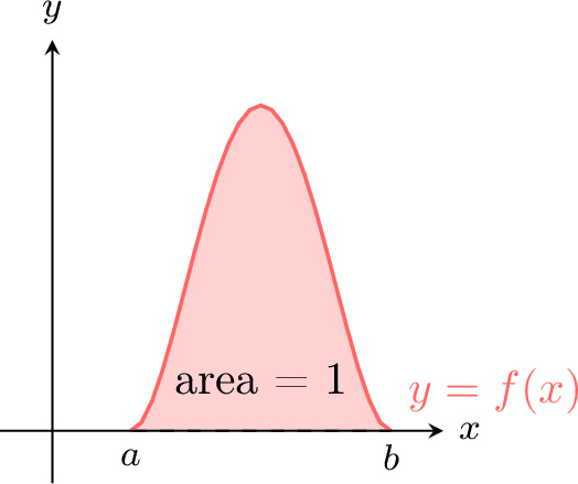
A function $f$ is a probability density function (pdf) on the interval $[a, b]$ if:

$f(x) \geq 0$ for all $x \in [a, b]$ (non-negative everywhere),
$\int_{a}^{b} f(x) \, dx = 1$ (the total area under the curve equals 1).

Example

The random variable $X$ takes values on $[0, 2]$ with density $f(x) = \frac{x}{2}$.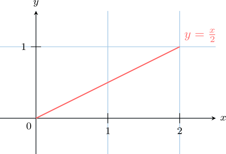

Verify that $f$ is a probability density function on $[0, 2]$.

Answer

$f(x) = \frac{x}{2} \geq 0$ for all $x \in [0,2]$, since $x \geq 0$.
Compute the total area: $$ \begin{aligned}[t] \int_{0}^{2} f(x) \, dx &= \int_{0}^{2} \frac{x}{2} \, dx \\ &= \left[ \frac{x^2}{4} \right]_{0}^{2} \\ &= \frac{2^2}{4} - 0 = 1 \end{aligned} $$ Since both conditions hold, $f(x) = \frac{x}{2}$ is a valid pdf on $[0, 2]$.

Definition Density of a Continuous Random Variable

A random variable $X$ with values on $[a, b]$ has a density $f$, if the probability that $X$ lies between $c$ and $d$ ($c, d \in [a, b]$) is:$$P(c \leq X \leq d) = \int_{c}^{d} f(x) \, dx$$This represents the area under the curve $y = f(x)$ from $x = c$ to $x = d$.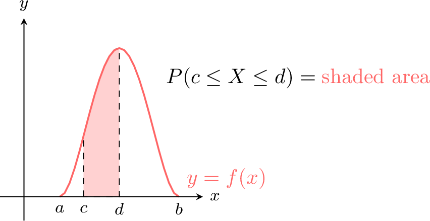

Remark

Since $f(x) \geq 0$, $P(c \leq X \leq d) \geq 0$.
Since $\int_{a}^{b} f(x) \, dx = 1$, $P(a \leq X \leq b) = 1$.

Example

The random variable $X$ with values on $[0, 2]$ has density $f(x) = \frac{x}{2}$. Find $P(1 \leq X \leq 2)$.

Answer

$$\begin{aligned}[t]P(1 \leq X \leq 2) &= \int_{1}^{2} \frac{x}{2} \, dx \\ &= \left[ \frac{x^2}{4} \right]_{1}^{2} \\ &= \frac{2^2}{4} - \frac{1^2}{4} \\ &= 1 - \frac{1}{4}\\ &= \frac{3}{4}\end{aligned}$$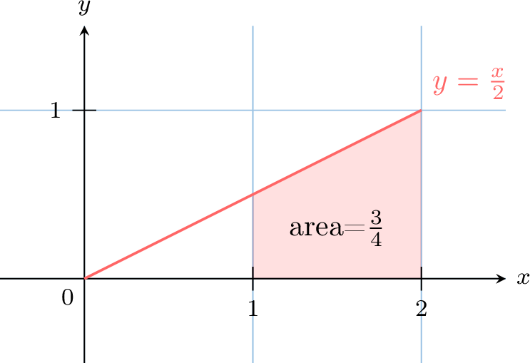

Expectation

The expectation (or expected value) of a continuous random variable is the "average" value it would take if the experiment were repeated infinitely. It represents the center of the distribution and is calculated as a weighted average, where the pdf $f(x)$ provides the weighting:$$\begin{aligned}[t]E(X)&=\sum_{x\in[a,b]}x P(x \leqslant X < x+\mathrm d x)\\ &=\sum_{x\in[a,b]}x \dfrac{P(x \leqslant X < x+\mathrm d x)}{\mathrm d x}\mathrm d x\\ &=\int_{a}^b xf(x)\;\mathrm d x\\ \end{aligned}$$

Definition Expectation

For a continuous random variable $X$ with density $f$ on $[a, b]$, the expected value is $$E(X) = \int_{a}^{b} x f(x) \, dx.$$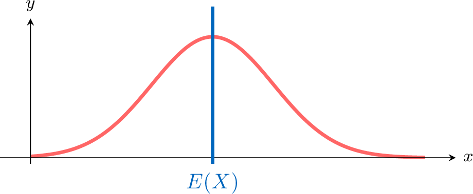

Example

The random variable $X$ with values on $[0, 3]$ has density $f(x) = \frac{x^2}{9}$: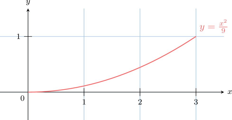

Find $E(X)$.

Answer

Compute $E(X)$: $$ \begin{aligned}[t] E(X) &= \int_{0}^{3} x \cdot \frac{x^2}{9} \, dx \\ &= \int_{0}^{3} \frac{x^3}{9} \, dx \\ &= \left[ \frac{x^4}{36} \right]_{0}^{3} \\ &= \frac{3^4}{36} - 0 \\ &= 2.25 \end{aligned} $$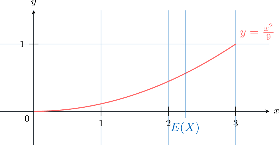

Example

The random variable $X$ with values on $[0,2]$ has density $f(x) = \frac{x}{2}$:

Find $E(X)$.

Answer

Compute $E(X)$:$$\begin{aligned}[t]E(X) &= \int_{0}^{2} x \cdot \frac{x}{2} \, dx \\ &= \int_{0}^{2} \frac{x^2}{2} \, dx \\ &= \left[ \frac{x^3}{6} \right]_{0}^{2} \\ &= \frac{2^3}{6} - 0 \\ &= \frac{8}{6} \\ &= \frac{4}{3} \\ \end{aligned}$$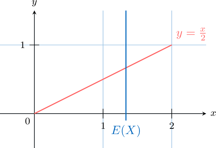

Variance

The variance of a continuous random variable measures the spread of its values around the expected value if the experiment were repeated infinitely. It quantifies the distribution’s dispersion and can be calculated as for a discrete random variable:$$\begin{aligned}[t]V(X) &= \sum_{x \in [a, b]} (x - E(X))^2 P(x \leq X < x + dx) \\ &= \sum_{x \in [a, b]} (x - E(X))^2 \frac{P(x \leq X < x + dx)}{dx} \cdot dx \\ &= \int_{a}^{b} (x - E(X))^2 f(x) \, dx\end{aligned}$$

Definition Variance and Standard Deviation

For a continuous random variable $X$ with density $f$ on $[a, b]$, the variance is$$V(X) = \int_{a}^{b} (x - E(X))^2 f(x) \, dx.$$The standard deviation is$$\sigma = \sqrt{V(X)}.$$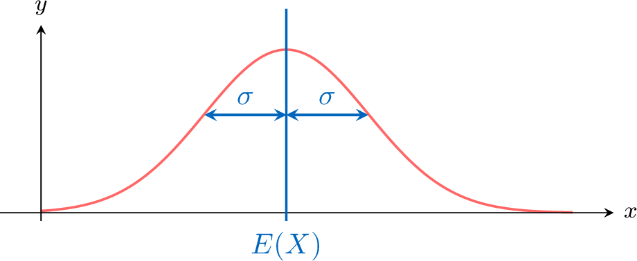

Proposition Computational Formula for Variance

A more convenient formula for variance computation is:$$V(X) = E(X^2) - [E(X)]^2$$

Example

The random variable $X$ with values on $[0,2]$ has density $f(x) = \frac{x}{2}$.
Find $V(X)$.

Answer

Compute $E(X)$: $$ \begin{aligned}[t] E(X) &= \int_{0}^{2} x \cdot \frac{x}{2} \, dx \\ &= \int_{0}^{2} \frac{x^2}{2} \, dx \\ &= \left[ \frac{x^3}{6} \right]_{0}^{2} \\ &= \frac{2^3}{6} - 0 \\ &= \frac{8}{6} \\ &= \frac{4}{3} \\ \end{aligned} $$
Compute $\int_{0}^{2} x^2 \cdot f(x) \, dx$: $$ \begin{aligned}[t] \int_{0}^{2} x^2 \cdot f(x) \, dx &=\int_{0}^{2} x^2 \cdot \frac{x}{2} \, dx\\ &= \int_{0}^{2} \frac{x^3}{2} \, dx \\ &= \left[ \frac{x^4}{8} \right]_{0}^{2} \\ &= \frac{2^4}{8} - 0 \\ &= \frac{16}{8} \\ &= 2 \end{aligned} $$
Compute $V(X)$ using the alternative formula: $$ \begin{aligned}[t] V(X) &= \int_{0}^{2} x^2 \cdot f(x) \, dx - [E(X)]^2 \\ &= 2 - \left(\frac{4}{3}\right)^2 \\ &= 2 - \frac{16}{9} \\ &= \frac{18}{9} - \frac{16}{9} \\ &= \frac{2}{9} \end{aligned} $$

Classical Distributions

Continuous Uniform Distribution

The continuous uniform distribution applies to events that are equally likely across an interval, such as the spinner example. The density is constant over the range.

Definition Continuous Uniform Distribution

A continuous random variable $X$ follows a continuous uniform distribution on $[a, b]$ if its density is:$$f(x) = \frac{1}{b - a} \quad \text{for} \quad a \leq x \leq b$$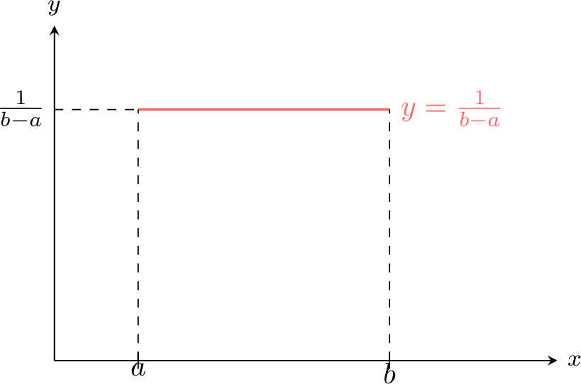

Proposition Properties

Let $ X $ be a continuous random variable following a continuous uniform distribution on $[a, b]$:

for all $ c, d \in [a, b] : P(c \leq X \leq d) = \frac{d - c}{b - a}$,
$E(X) = \frac{a + b}{2}$.
$V(X) = \frac{(b-a)^2}{12}$.

Proof

Probability: $$ \begin{aligned}[t] P(c \leq X \leq d) &= \int_{c}^{d} \frac{1}{b - a} \, dx \\ &= \left[ \frac{x}{b - a} \right]_{c}^{d} \\ &= \frac{d - c}{b - a} \end{aligned} $$
Expected value: $$ \begin{aligned}[t] E(X) &= \int_{a}^{b} x \cdot \frac{1}{b - a} \, dx \\ &= \left[ \frac{x^2}{2(b - a)} \right]_{a}^{b} \\ &= \frac{b^2 - a^2}{2(b - a)}\\ &= \frac{(b - a)(b + a)}{2(b - a)}\\ &= \frac{a + b}{2} \end{aligned} $$
Variance: We use the formula $V(X) = E(X^2) - [E(X)]^2$. First, we compute $E(X^2)$. $$ \begin{aligned}[t] E(X^2) &= \int_{a}^{b} x^2 \cdot \frac{1}{b-a} \, dx \\ &= \frac{1}{b-a} \left[ \frac{x^3}{3} \right]_{a}^{b} \\ &= \frac{b^3-a^3}{3(b-a)} = \frac{(b-a)(b^2+ab+a^2)}{3(b-a)} = \frac{a^2+ab+b^2}{3} \end{aligned} $$ Now we can compute the variance: $$ \begin{aligned}[t] V(X) &= \frac{a^2+ab+b^2}{3} - \left(\frac{a+b}{2}\right)^2 \\ &= \frac{4(a^2+ab+b^2) - 3(a+b)^2}{12} \\ &= \frac{4a^2+4ab+4b^2 - 3(a^2+2ab+b^2)}{12} \\ &= \frac{4a^2+4ab+4b^2 - 3a^2-6ab-3b^2}{12} \\ &= \frac{a^2-2ab+b^2}{12} = \frac{(b-a)^2}{12} \end{aligned} $$

Exponential Distribution

Proposition Probability Density Function

Let $\lambda$ be a strictly positive real number.
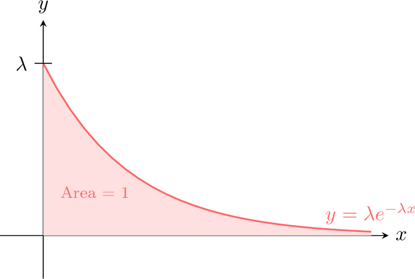
The function $f$ defined on $[0, +\infty)$ by $f(x) = \lambda e^{-\lambda x}$ is a probability density function on $[0, +\infty)$.

Definition Exponential Distribution with Parameter $\lambda$

We call the exponential distribution with parameter $\lambda > 0$, denoted $\mathcal{E}(\lambda)$, the probability distribution whose density is the function $f$ defined on $[0, +\infty)$ by $f(x) = \lambda e^{-\lambda x}$.

Remark

$f(0) = \lambda e^{-\lambda \times 0} = \lambda e^0 = \lambda$. Therefore, the $y$-intercept of the representative curve of $f$ is equal to $\lambda$.

Proposition Calculating Probabilities

For any positive numbers $a$, $c$, and $d$:

$P(X \leq a) = 1 - e^{-\lambda a}$
$P(X \geq a) = e^{-\lambda a}$
$P(c \leq X \leq d) = e^{-\lambda c} - e^{-\lambda d}$

Proof

$\displaystyle P(X \leq a) = \int_{0}^{a} \lambda e^{-\lambda x} dx = \left[ -e^{-\lambda x} \right]_{0}^{a} = -e^{-\lambda a} - (-e^{-\lambda \times 0}) = -e^{-\lambda a} + e^0 = 1 - e^{-\lambda a}$.
$P(X \geq a) = 1 - P(X < a) = 1 - P(X \leq a) = 1 - (1 - e^{-\lambda a}) = e^{-\lambda a}$.
$\displaystyle P(c \leq X \leq d) = \int_{c}^{d} \lambda e^{-\lambda x} dx = \left[ -e^{-\lambda x} \right]_{c}^{d} = -e^{-\lambda d} - (-e^{-\lambda c}) = e^{-\lambda c} - e^{-\lambda d}$.

Proposition Expectation

The expected value of a random variable $X$ following an exponential distribution with parameter $\lambda$ is:$$E(X) = \frac{1}{\lambda}$$

Proposition Memoryless Property

Let $X$ be a random variable following an exponential distribution with parameter $\lambda > 0$. For all strictly positive numbers $x$ and $h$:$$P_{X>x}(X > x+h) = P(X > h)$$ This means the probability of lasting $h$ more units of time does not depend on how much time $x$ has already passed.

Example

Let the lifespan of a device in years be a random variable following an exponential distribution with parameter $\lambda = 0.1$.
We have $P_{X>3}(X > 5) = P_{X>3}(X > 3 + 2) = P(X > 2)$.
So, if the device has already functioned for more than 3 years, the probability that it functions for 2 more years (totaling more than 5 years) is the same as the (unconditional) probability of functioning for more than 2 years from the start.